Data
Prevision.io allows you to import data into your environment for further processing. Data can come from remote persistent sources (e.g. SQL database, HIVE…) or can be imported directly (e.g. CSV data, ZIP,…)
To carry out the import of data, we distinguish between 4 notions:
Data Sets: a data set that can be a snapshot of a data source at a given time or simply a CSV or ZIP imported directlyImage folders: a data folder containing images set that can come from a ZIP imported directlyData Sources: a connector completed by a query, a base / table, a pathConnectors: a pointer to a persistent external environment containing data
Data Sets
Data Sets are data that can be manipulated in Prevision.io. They are in tabular form and are derived:
- Either from files (CSV, ZIP)
- Either from a Data Source at a given time (snapshot)
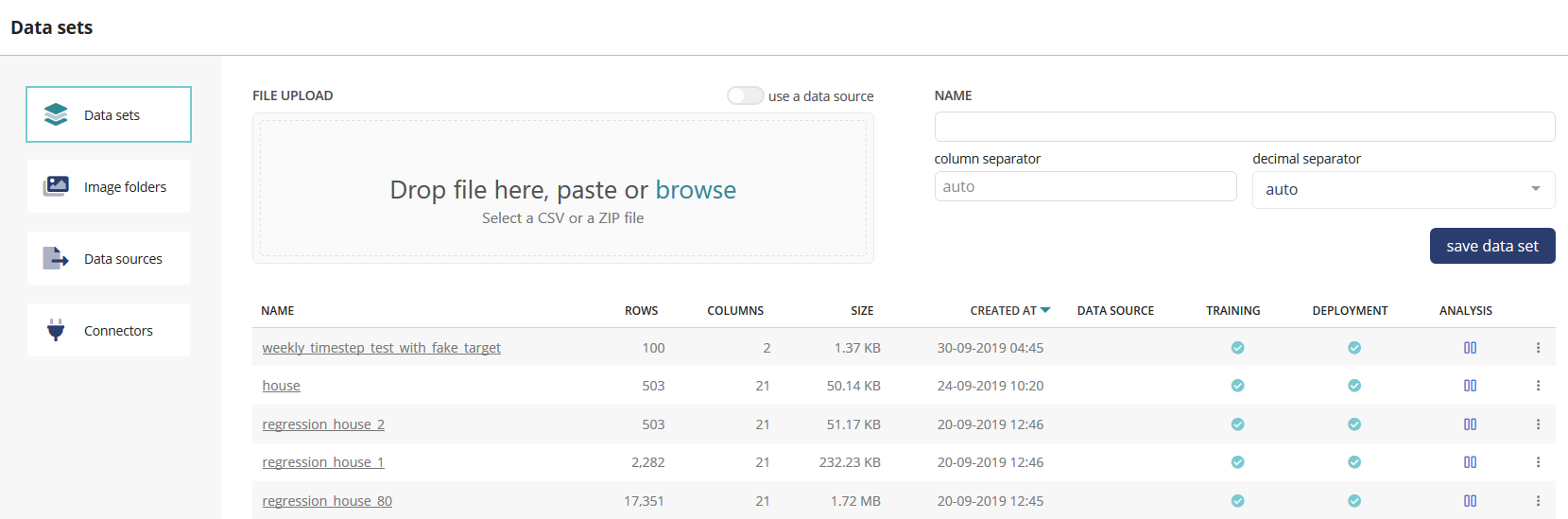
All Data Sets are presented in a table with their main characteristics.
By clicking on the … at the far right of the table, it is also possible to:
- Edit the Data Set name
- Download the Data Set in a ZIP
- Start analysis of the Data Set
- Remove the Data Set
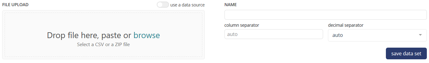
Create a Data Set from a local file
To create a new Data Set from a local, simply drag n” drop a file in the upper left box (or browse for it). CSV file and ZIP containing one CSV file are supported.
You can then choose the Data Set name and select separators before saving the Data Set. Please note that the auto detection should work in most cases.
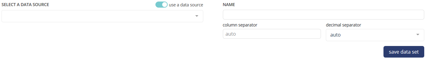
Create a Data Set from a Data Source
If you want to snapshot a previously created Data Source, simply create a Data Set from it. No additional information is required, except the name you wish to give to the Data Set.
Once created
The Data Set name will appears in the bottom table. We will display :
Data Set name
Number of rows
Number of columns
Size
Date of creation
If it is linked to a Data Source
A parsed indicator :
- Spinning : Data Set is beeing processed for training / prediction (checking it is tabular, checking data types, …)
- Green : Data Set is ready for beeing trained / predicted on
- Red : Data Set can’t be trained / predicted on. This is blocking and indicates a structural error on it
A deployment indicator :
- Spinning : Data Set is beeing processed for deployment (calculating drift)
- Green : Data Set is ready for beeing deployed once a model has been trained on it
- Red : Data Set drift can’t be monitored if a use case linked to it is deployed (= non blocking)
An analysis indicator :
- Paused : Data Set has no analysis done on it (default behavior - it can’t be seen in the Data Explorer)
- Spinning : Data Set analysis is beeing computed
- Green : Data Set can be analysed in the Data Explorer
- Red : Data Set can’t be analysed in the Data Explorer because of an error
A
...menu allowing you to :- Edit the Data Set name
- Create a use case from the Data Set
- Start / Stop / Explore the Data Set
- Download the Data Set
- Remove the Data Set
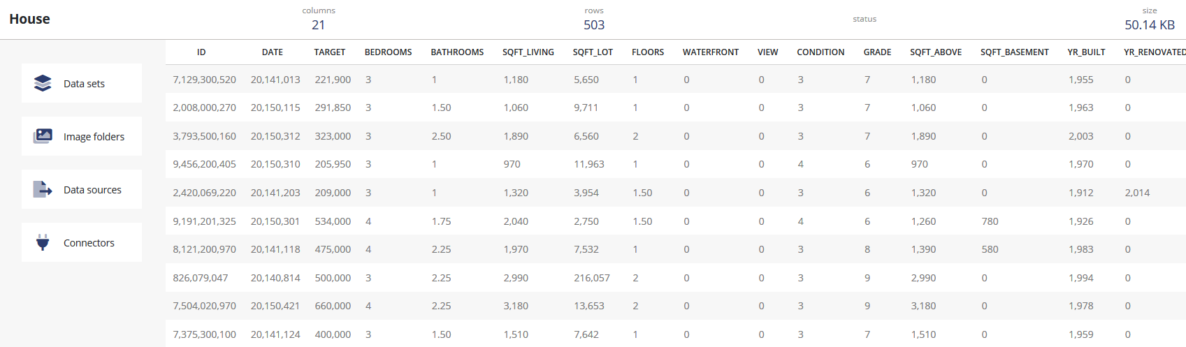
Also, a click on the Data Set name will display the top 10 rows of it :
Dataset page
In this screen you’ll find:
General information about the dataset:
- Number of features
- Number of rows
- Number of cells (rows * features)
- Number of missing value (%)
Feature type distribution
Correlation matrix (top correlation only)
Macro analysis of features
- Feature name
- Feature type
- % of missing values in the dataset
Data Explorer
The Data Explorer is a specific module that aim to detect similarities between samples of your dataset. It uses a combination of Dimension reduction algorithms for representing your dataset into a vector space, sometimes called embedding By using it, you’re being able to :
- Visually observe cluster
- see wich samples are the most similar to a selected one, for exemple a Customer in his buying habits
- See in wich population a given feature, like expenses, is present or higher
- Have a global view of your data
The Data explorer is often use as a pre-analysis of dataset, as it uses unsupervised alogorithm, but it can be uses as a standalone feature. Once the embedding has been generated you can request them by API or download them for use in a thrd party tool like Excel.
Launching the analysis of a Data set
Embedding are generated from any dataset and should be manually launched, as they require computing power.
Once a tabular dataset have been uploaded in the data tab, your can launch an analysis.
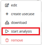
To do so, click on the ... icon located at the right of the row describing the selected Data set and click on start analysis
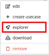
The analysis indicator will start spinning. Once green, the Data set can be seen in the Data Explorer. To do so, click on the ... icon located at the right of the row describing the selected Data set and click on explorer
The Explorer
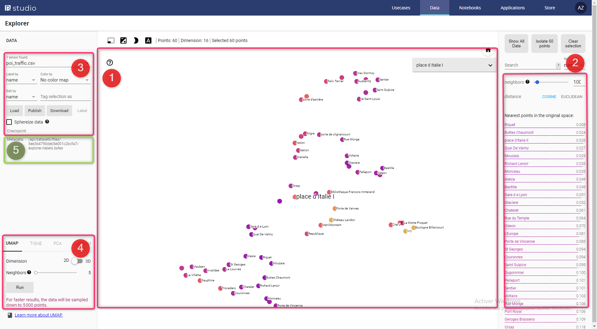
The Data Explorer is now accessible and will give you a visual representation in 2 or 3 dimensions of the selected Data Set. This representation is a dimention reduction constrained to 2 or 3 dimension, apply on the embedded vectors, that may be of an higher dimension. There are five important section in the data explorer.
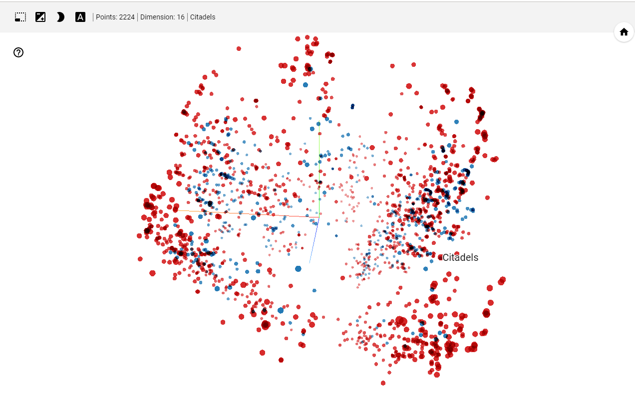
(1) Graphical projection
The main screen is a visual representation of the dataset. Each point is a sample of your dataset ( up to 5000 ). You can pan and zoom and if you click on a point, or use the selecting box tool, some more info are displayed.
In this representation, point are group by similarities as much as possible, meaning that if two points are near in this space, the samples share some important similarities.
The nature of the displayed information are selected on the section (3)
(2) Search and similarities
The second section is a dynamic list of similar sample.
You can search any sample from any feature. For example if your dataset has an index with name, you can search a sample by using its name but you can too search all the sample that have « RPG » as type or « 5 » for size.
Once a sample is selected, it and a list of similar are is highlighted in the main section. They can be further isolated by clicking on the « isolate N points » button on top of the section..
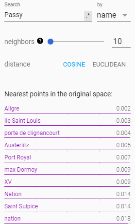
The number of similar samples to display can be choosen with the « neighbors » slider

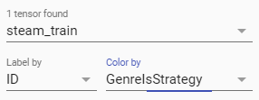
(3) Labels
Section 3 main purpose is to set labels displayed in section 1. Here you can set :
- the label displayed above each point
- the feature use for coloring each point :
(4) Segmenting and clustering
Section 4 is all about Segmenting and clustering your samples.
Here you can choose an algorithm and tune its parameter to display the most similar point together. Thus, you can start to observe sample cluster, or segment of data that represent big group that share important similarities.
Yet, as we try to project a lot of dimension in a smaller space (3D or 2D), note that this algorithm are just for display and shaping human decision. A lot of the process is a little bit subjective and further conclusion should be driven by a supervised algorithm.
Anyway, here you can choose between 3 algorithms :
- PCA : the quickest and simplest algorithm. Clicking on the PCA tab immediately led to a 3D representation of your samples. Yet, this is a very simple algorithm that only show sample variability along 3 axes.
- T-SNE : once you click on the T-SNE tab, a process of convergence is launched. T-SNE is a very time consuming algorithm but that can lead to very accurate segmentation. You can change its parameters and click on « Stop » button then « Re-run » it. But in most of case it’s better to already know this algorithm to use it.
- UMAP : UMAP is a good alternative to T-SNE and PCA. Quicker than T-SNE , it offers better result thant PCA. THe only parameters is « Neighbors », that change the size of clusters. The more neighbors you ask for, the bigger the cluster.
We recommend to use UMAP in most of case.
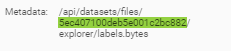
(5) API informations
The 5th part is only about API informations.
When launching a dataset Analysis, the platform built an embedding of dataset, namely, it projects each sample of the dataset to a vector. This embedding is attached to the dataset and can be retreived wit the dataset ID. Then you can use it for running any mathematical operation, in most of case a distance, that can be ran on vectors.
Section 5 of the tools gives you the Id of your dataset :
With it you can access several URL :
- GET https://<YOUR_DOMAIN>.prevision.io/api/datasets/files/<DATASET_ID>/download : get the original dataset
- GET https://<YOUR_DOMAIN>.prevision.io/api/datasets/files/<DATASET_ID> : JSON info about your dataset
- GET https://<YOUR_DOMAIN>.prevision.io/api/datasets/files/<DATASET_ID>/explorer : JSON info about the embeddding
- GET https://<YOUR_DOMAIN>.prevision.io/api/datasets/files/<DATASET_ID>/explorer/tensors.bytes : numpy files of embeddings
- GET https://<YOUR_DOMAIN>.prevision.io/api/datasets/files/<DATASET_ID>/explorer/labels.bytes : tsv files of labels
The embedding files (tensor.bytes) is a numpy float 32 file whom shape is in the json file if explorer URL. You can read it with the following python code for example :
1 2 3 4 5 | req = Request('https://<YOUR_DOMAIN>.prevision.io/ext/v1/datasets/files/<DATASET_ID>/explorer/tensors.bytes')
req.add_header('Authorization',<YOUR_TOKEN> ) #get YOUR_TOKEN in the admin page
content = urlopen(req).read()
vec = np.frombuffer(BytesIO(content).read(), dtype="float32").reshape(u,v) # u,v is the shape gotten in /ext/v1/datasets/files/<DATASET_ID>/explorer
print(vec.shape)
|
Please note that you can use SDK’s functions in order to simplifies this process.
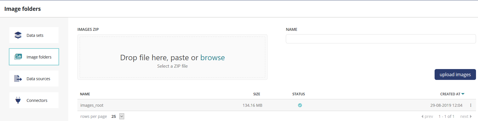
Image Folders
An Image Folder is a ZIP containing 1 to n images that will be needed for training image use cases.
The process of creating an Image Folder is similar compared to a Data Set. However, less analytics will be computed on it because of its nature.
Data Sources
Data Sources require the existence of a connector, which is supplemented by information in order to point to a specific data source (query, database + table, file name, …)
All Data Sources are presented in a table with their main characteristics.
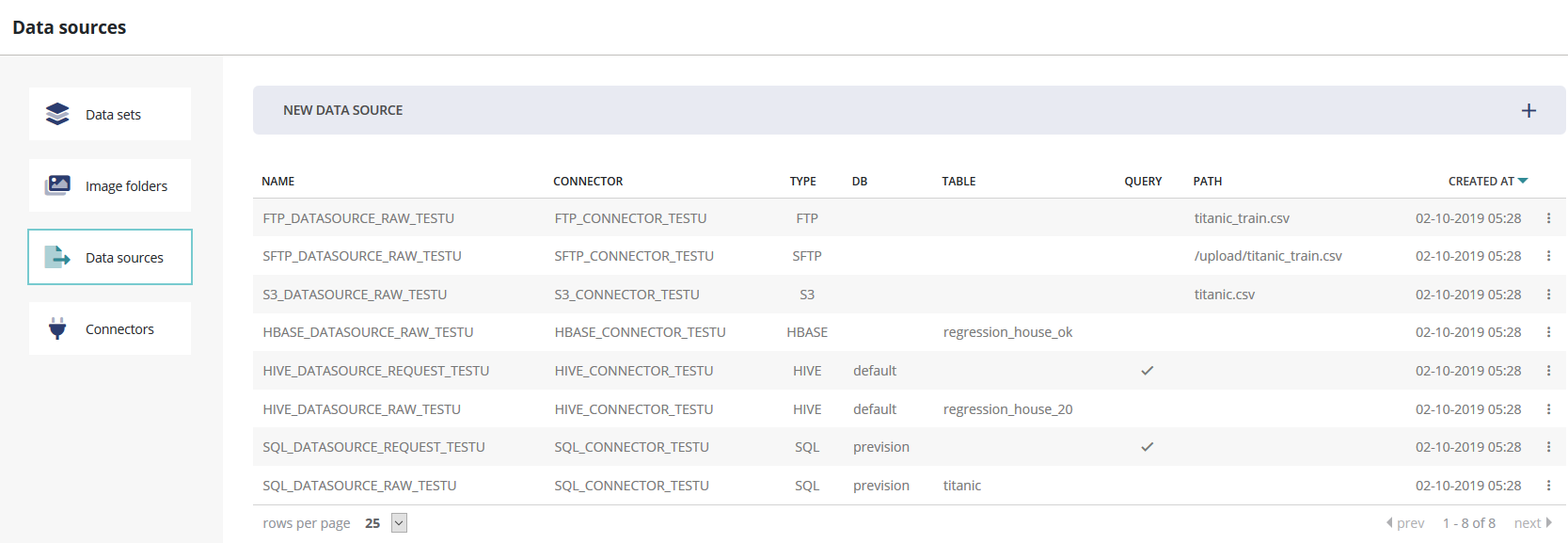
This table is completed by 3 possible actions:
- Test a Data Source
- Edit a Data Source
- Remove a Data Source
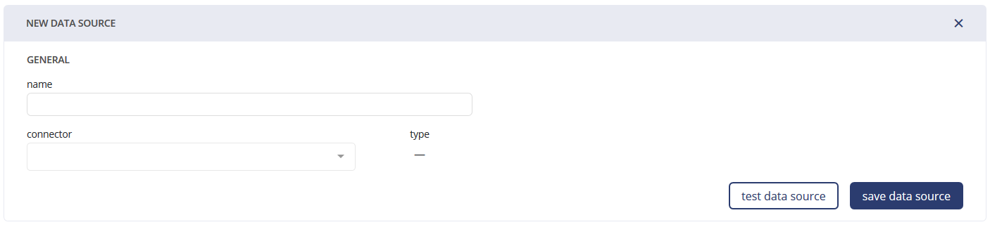
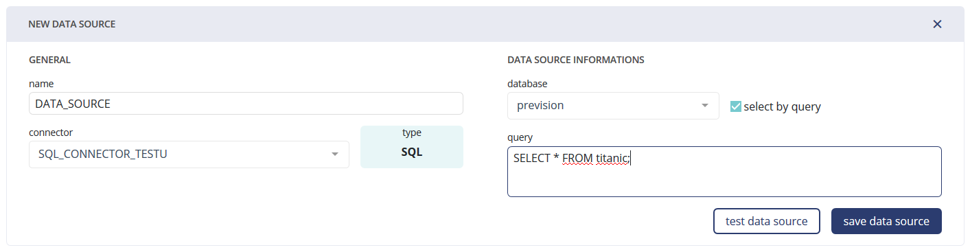
To create a Data Source, simply click on the « New Data Source » button.
For Data Sources from database connectors, it is possible to request via drop-down lists the database and table of your choice
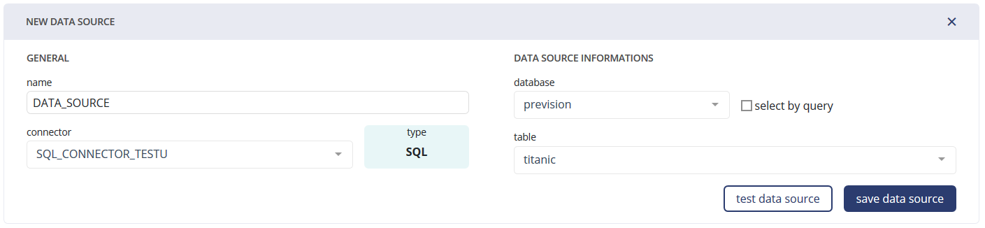
For Data Sources from SQL and HIVE connectors, it is also possible to choose a database and write a SQL query if you require more modularity:
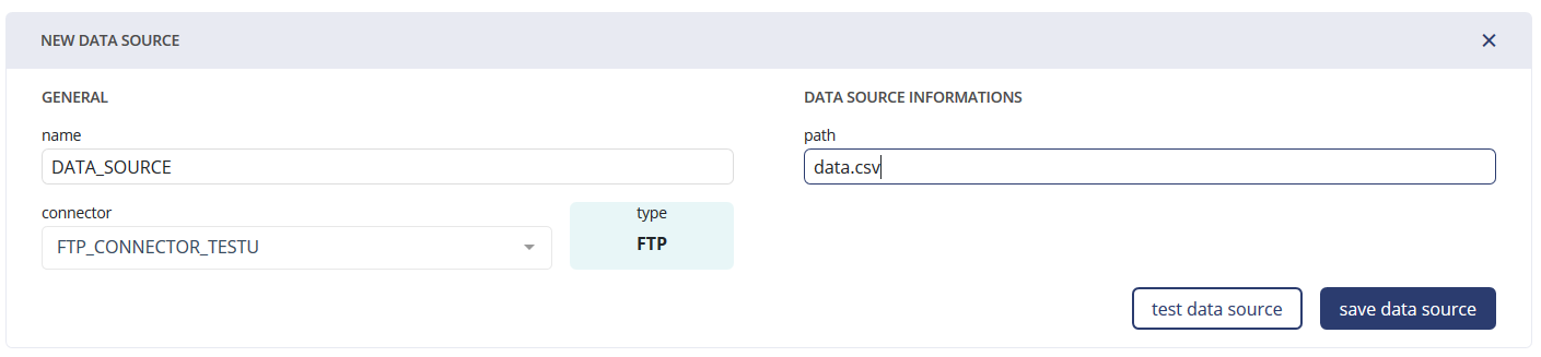
For Data Sources from FTP connectors, a file path must be filled in
Connectors
Connectors are pointers to persistent data sources. Several types of connectors are currently supported by Prevision. To know:
- SQL
- HIVE
- HBASE
- FTP
- SFTP
- S3
All connectors are presented in a table with their main characteristics (please note that host have been remove in the following screenshot)
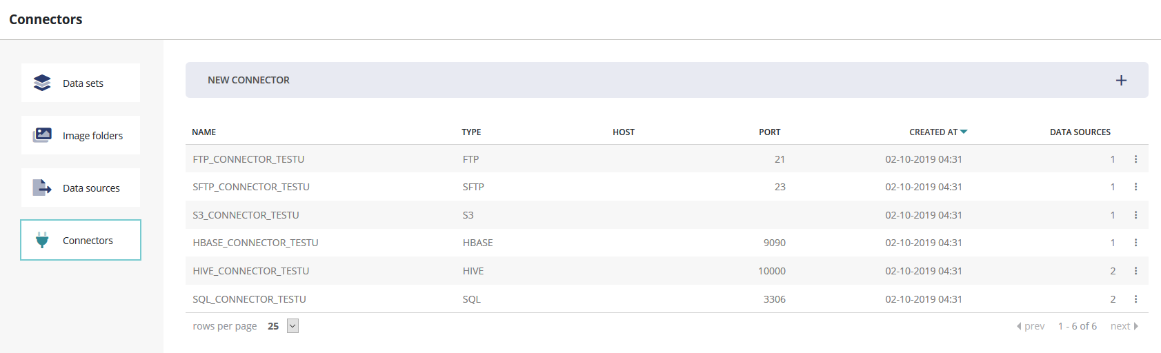
This table is completed by 3 possible actions:
- Test the connector
- Edit the connector
- Remove the connector
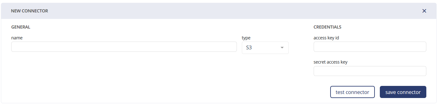
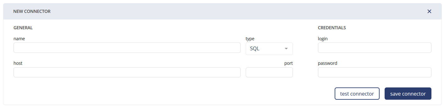
To create a connector, simply click on the « New Connector » button.
Connection to databases such as SQL - HIVE - HBASE - HBASE - FTP - SFTP is possible with the following information:
- Name: The name of your connector
- Type: The desired connector type
- Host: The URL to your environment
- Port: The port to your environment
- Login: The login allowing you to connect to your environment
- Password: The password to connect to your environment
Connection to data stored on Amazon S3 is possible with the following information:
- Login: Your Access_Key_ID
- Password: Your Access_Key