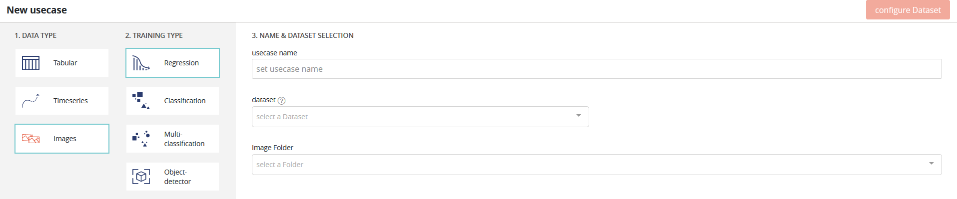
New usecase
In order to create a new usecase, from the usecase tab, you need to click on the « new usecase » button:

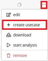
You can also create directly a usecase by clicking the … icon near a given Data set in the data screen :
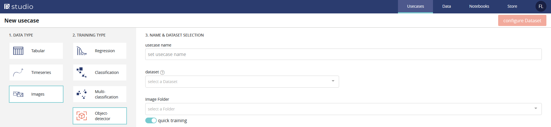
When creating a new usecase, you should first specify a DATA TYPE among:
- Tabular (including textual)
- Time series
- Images
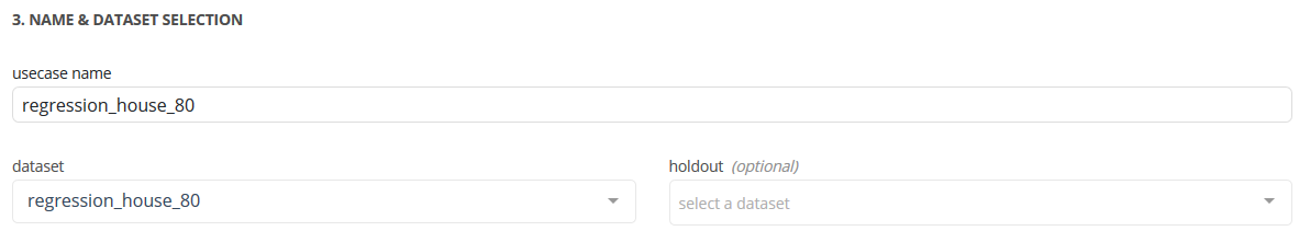
Then, you can specify a usecase name linked to a previously created Data Set.
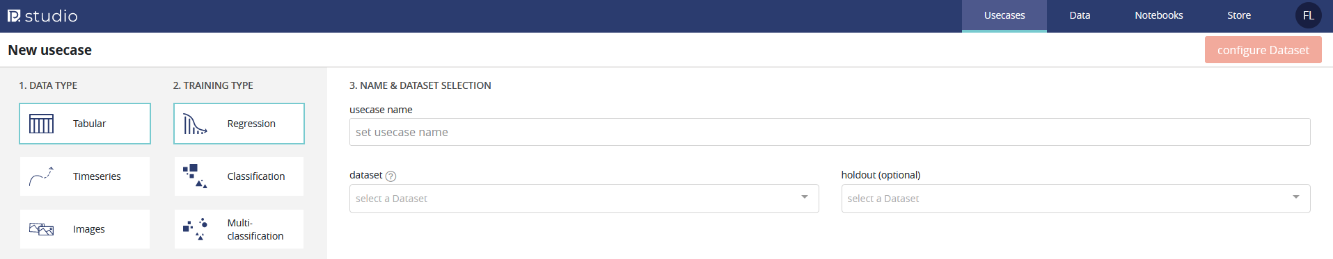
Depending on the TRAINING TYPE, some options are displayed :
- Hold out : only for Tabular usecases. It is a Data Set that will be predicted for each model trained and the performance will be compute on it
- Image folder : only for Images usecases. It is a Data Set labelled as a folder containing images linked to a tabular Data Set
We offer 4 differents TRAINING TYPE:
| TYPE | TABULAR | TIMESERIES | IMAGE | DEFINITION | EXAMPLE |
| Regression | OK | OK | OK | Prediction of a quantitative feature | 2.39 / 3.98 / 18.39 |
| Classification | OK | OK | Prediction of a binary quantitative feature | « Yes » / « No » ou 0 / 1 | |
| Multi classification | OK | OK | Prediction of a qualitative feature whose cardinality is > 2 | « Victory » / « Defeat » / « Tie game » | |
| Object detection | OK | Detection from 1 to n objects per image + location | Is there a train on this image ? If so, where ? |
Tabular
The screens for these 3 types of usecases are extremely similar. Only metrics, detailed below, change according to the type of project. First, you should give your usecase a name and attach a previously created Data Set:
Note that only tabular Data Sets with an OK parsed status (✓ icon on the Data Set screen on the PARSED column) are selected.
It is also possible, but not mandatory, to add a Data Set for comparison (hold out):
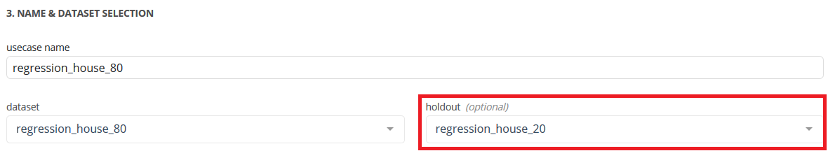
Typically, the addition of such a Data Set is useful in a study context in which we want to compare the quality of the actual prediction (and no longer only the performance estimators) on a set of models. This Data Set must have the same structure as the original set (same column name).
Once this step done you can proceed on cliquing the configure dataset button, located on the top right of the screen:

Data Set configuration
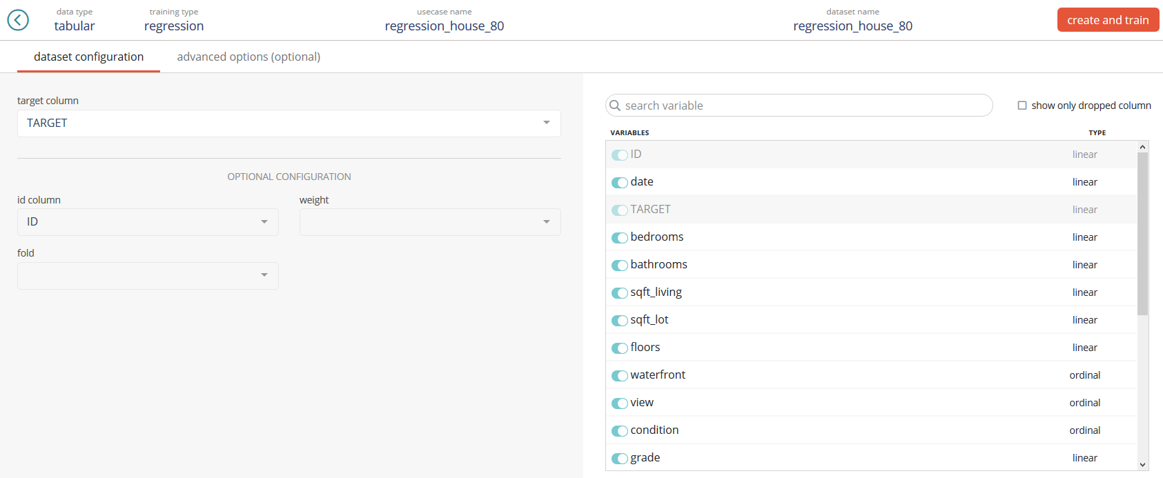
On the left part of the screen, you will be able to fill:
- The target column (mandatory). This column is the one we want to predict on.
- The id column (optionnal). This column has typically no predictive power and is used to make join on other Data Sets later on.
- The fold (optionnal). Typically, this column will contain a feature of 1, 2, … n (n being the maximum number of folds). If fed, the CV stratification will be based on this column and won’t be stratified to the target which is Prevision.io’s default behavior.
- The weight (optionnal). Typically, this column contains a linear feature indicating the importance of a given row. The higher the weight, the more important the row is. If not fed, all rows are considered equally important (which is the case in most usecases).
Note: If your Data Set contains a column named ID or TARGET, these will automatically be detected and selected from the corresponding menus
On the right part of the screen, you will be able to:
- Filter columns by names
- Shows only dropped (removed) columns
- Drop (remove) columns for the training phase. This means that every dropped column won’t be use in the learning process
Once done, you can launch the training by clicking on the create and train button, located on the top right of the screen:

Optionnally, there are advanced options reachable by clicking the tab in the top bar:

Advanced options
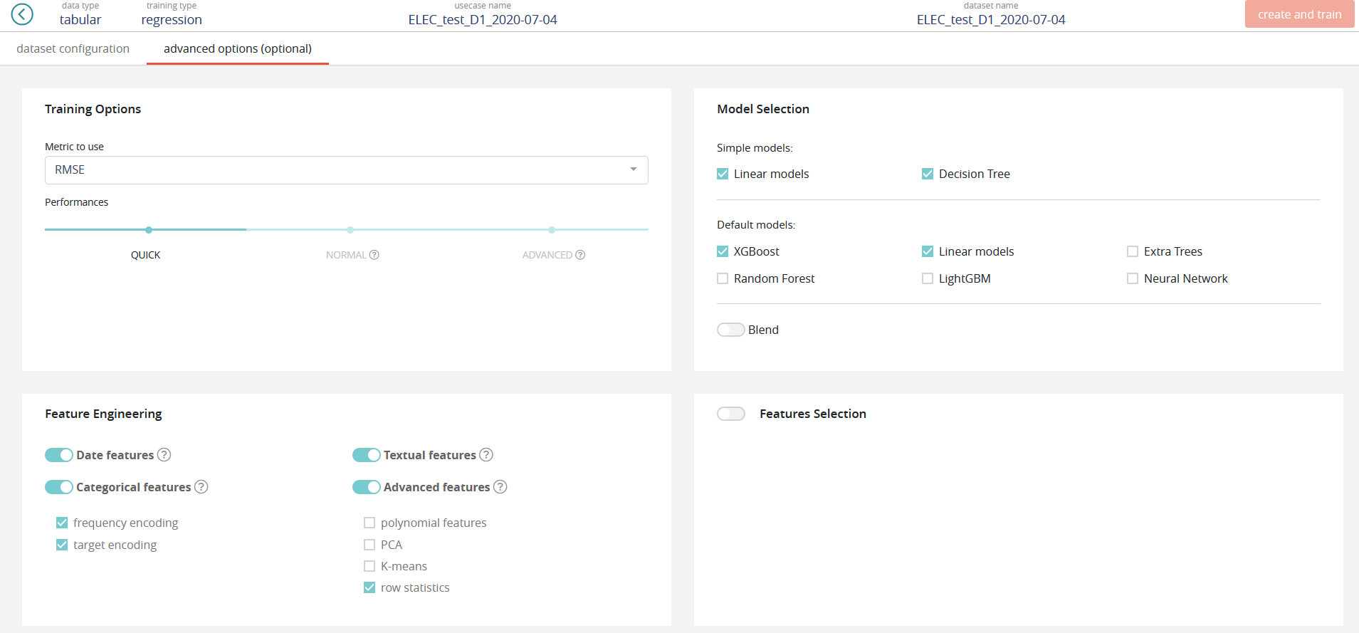
Training options
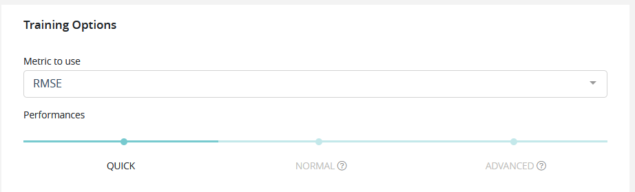
In this part of the screen, you can tune the following:
Metric (will differ depending of the training type):
| TYPE | METRIC | DEFINITION | DEFAULT ? |
| Regression | RMSE | Root mean squared error | YES |
| Regression | MSE | Mean squared error | |
| Regression | RMSLE | Root mean squared logarithmic error | |
| Regression | RMSPE | Root mean squared percentage error | |
| Regression | MAE | Mean absolute error | |
| Regression | MAPE | Mean absolute percentage error | |
| Regression | MER | Median absolute error | |
| Regression | R2 | Coefficient of determination | |
| Regression | SMAPE | Symetric mean absolute percentage error | |
| Classification | AUC | Area under ROC curve | YES |
| Classification | ERROR RATE | Error rate | |
| Classification | LOGLOSS | Logarithmic loss | |
| Classification | ACCURACY | Accuracy | |
| Classification | F05 | F-0.5 Score | |
| Classification | F1 | F-1 Score | |
| Classification | F2 | F-2 Score | |
| Classification | F3 | F-3 Score | |
| Classification | F4 | F-4 Score | |
| Classification | MCC | Matthews” correlation coefficient | |
| Classification | GINI | Gini’s coefficient | |
| Classification | AUPCR | Area under precision-recall curve | |
| Classification | LIFT_AT_0.1 | Lift @ 10% | |
| Classification | LIFT_AT_0.2 | Lift @ 20% | |
| Classification | LIFT_AT_0.3 | Lift @ 30% | |
| Classification | LIFT_AT_0.4 | Lift @ 40% | |
| Classification | LIFT_AT_0.5 | Lift @ 50% | |
| Classification | LIFT_AT_0.6 | Lift @ 60% | |
| Classification | LIFT_AT_0.7 | Lift @ 70% | |
| Classification | LIFT_AT_0.8 | Lift @ 80% | |
| Classification | LIFT_AT_0.9 | Lift @ 90% | |
| Multi classification | LOGLOSS | Logarithmic loss | YES |
| Multi classification | ERROR_RATE | Error rate | |
| Multi classification | AUC | Area under ROC cure (mean of AUC by class) | |
| Multi classification | MACROF1 | Macro F1-Score (mean of F1 by class) | |
| Multi classification | ACCURACY | Accuracy | |
| Multi classification | QKAPPA | Quadratic weighted Kappa | |
| Multi classification | MAP_AT_3 | Mean average precision @ 3 | |
| Multi classification | MAP_AT_5 | Mean average precision @ 5 | |
| Multi classification | MAP_AT_10 | Mean average precision @ 10 |
All technicals formulas are available here : https://previsionio.readthedocs.io/fr/latest/_static/ressources/formula.pdf
Performances:
- QUICK: Training is done faster but performance may be slightly lower. Ideal in iterative phase.
- NORMAL: Intermediate value, suitable for most usecases on a later stage.
- ADVANCED: The training is done in an optimal way. Though the performance will be more stable, the calculations will take longer to process. This is ideal when the model is put into production and the performance is discriminating.
Model Selection
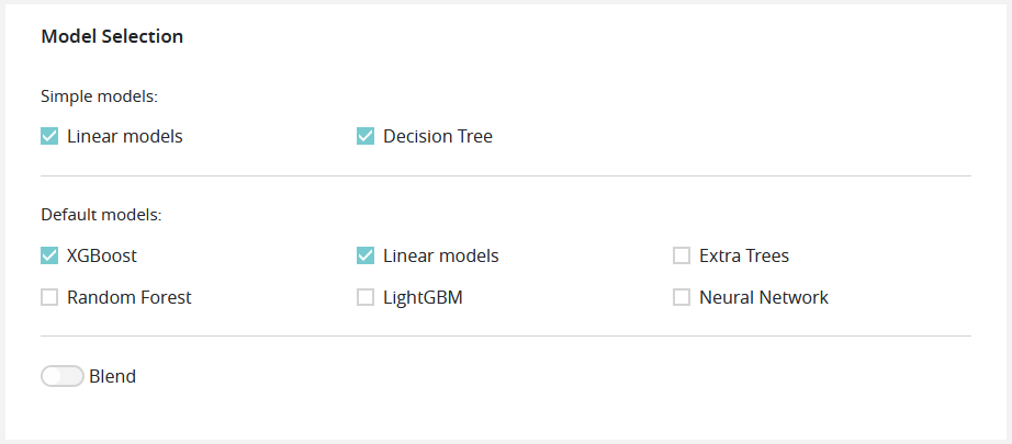
In this part of the screen you can enable or disable model types, such as:
Simple models (with simple feature engineering)
- Linear models (https://en.wikipedia.org/wiki/Linear_regression or https://en.wikipedia.org/wiki/Logistic_regression)
- Decition tree (https://en.wikipedia.org/wiki/Decision_tree_learning)
Default models (with advanced feature engineering)
- XGBoost (https://github.com/dmlc/xgboost)
- Linear models (https://en.wikipedia.org/wiki/Linear_regression or https://en.wikipedia.org/wiki/Logistic_regression)
- Random Forest (https://en.wikipedia.org/wiki/Random_forest)
- LightGBM (https://github.com/Microsoft/LightGBM)
- Extra Trees (https://en.wikipedia.org/wiki/Random_forest#ExtraTrees)
- Neural Network (https://en.wikipedia.org/wiki/Artificial_neural_network)
Note: The more model types you add in the training, the longer it will be.
Feature Engineering
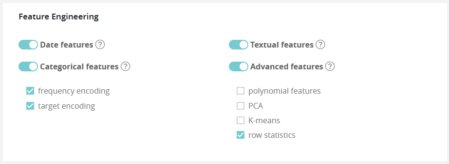
In this part of the screen you can enable or disable feature engineering, such as:
- Date features: dates are detected and operations such as information extraction (day, month, year, day of the week, etc.) and differences (if at least 2 dates are present) are automatically performed
- Textual features: Textual features: textual features are detected and automatically converted into numbers using 3 techniques:
By default, only TF-IDF approach is used.
Note
For better performance, it is advisable to check the word embedding and sentence embedding options. Checking its additional options will increase the time required for feature engineering, modeling, and prediction
Categorical features:
- Frequency encoding: modalities are converted to their respective frequencies
- Target encoding: modalities are replaced by the average (TARGET, grouped by modality) for a regression and by the proportion of the modality for the target’s modalities in the context of a classification
Advanced features:
- Polynomial features: features based on products of existing features are created. This can greatly help linear models since they do not naturally take interactions into account but are less usefull on tree based models
- PCA: main components of the PCA
- K-means: Cluster number comming from a K-means methode are added as new features
- Row statistics: features based on row by row counts are added as new features (number of 0, number of missing values, …)
Note: The more feature engineering you add in the training, the longer it will be.
Feature Selection
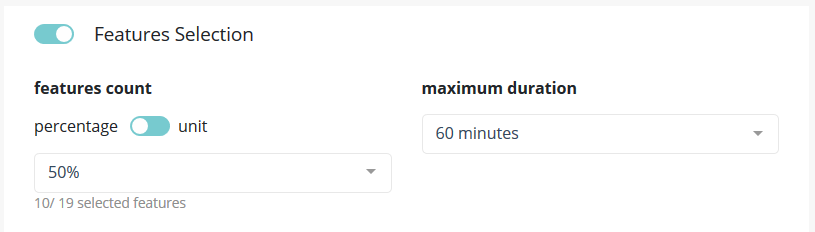
In this part of the screen you can chose to enable feature selection (off by default).
This operation is important when you have a high number of features (a couple hundreds) and can be critical when the number of features is above 1000 since the full Data Set won’t be able to hold in RAM.
You can chose to keep a percentage or a count of feature and you can give a time budget to Prevision.io’s to perform the search of optimal features given the TARGET and all other parameters. In this time, Prevision.io will subset the feature of the Data Set then start the classical process.
Time series
Time series is very similar to tabular usecase except:
- There is no hold out
- There is no weight
- There is no fold (in this case, Prevision.io use temporal stratification)
However, you will find some new notions:
Temporal column: the feature that contain the time reference of the time series. Since date formats can be complex, Prevision.io supports ISO 8601 (https://fr.wikipedia. org/wiki/ISO_8601) as well as standard formats (e.g. DD/MM/YYYY or DD-MM-YYYY hh:mm).
Time step: period between 2 events (within the same group) from the temporal column (automatically detected)
Observation window: illustrate the period in the past that you have for each prediction
- Start of observation window: the maximum time step multiple in the past that you’ll have data from for each prediction (inclusive, 30 by default)
- Enf of the observation window: the last time step multiple in the past that you’ll have data from for each prediction (inclusive, 0 by default that means that the immediate values before the prediction time step is known)
Prediction window: illustrate the period in the future that you want to predict
- Start of the prediction window: the first time step multiple you want to predict (inclusive, 1 by default which means we will predict starting at the next value)
- End of the prediction window: the last time stemp multiple you want to predict (inclusive, 10 by default which means we will predict up to the 10th next value)
A priori features: features whose value is known in the future (customer number, calendar, public holidays, weather…)
Group features: features that identify a unique time serie (e.g. you want to predict your sales by store and by product. If you have 2 stores selling 3 products, there are 6 time series in your file. Selecting features « store » and « product in the group column allows Prevision.io to take into account these multiple series)
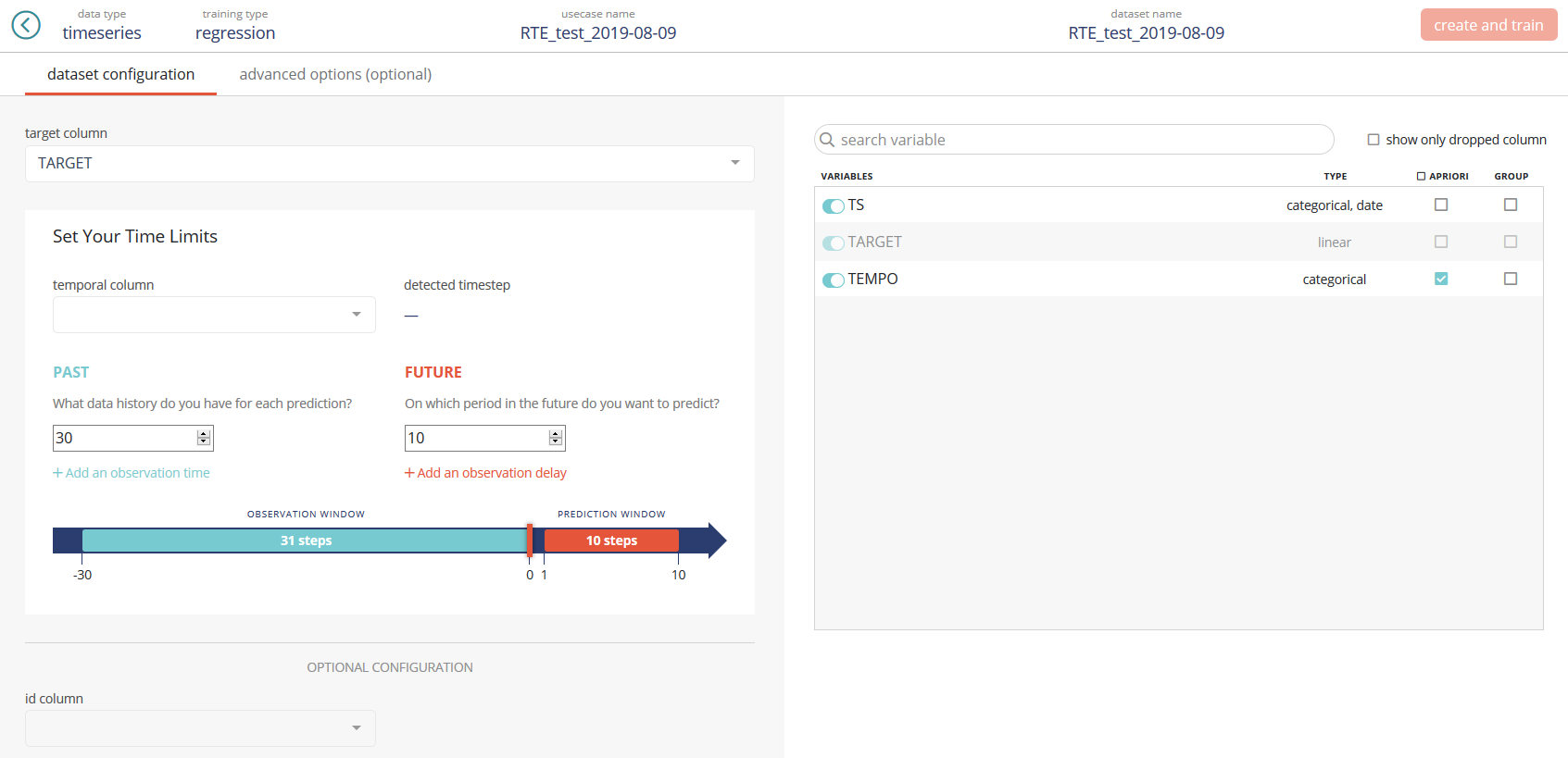
Once eveything set up, you can launch the training by clicking on the « create and train » button, located on the top right of the screen:
Optionnally, there are advanced options reachable by clicking the tab in the top bar:

Example 1 : You want to predict day ahead value per hour and you have all data available 1 week in the past for each value
Time step = 1 hour
Start of observation window = 7 (days) * 24 (hours / day) - 1 (because this value is inclusive) = 167
End of observation window = 0 (we have the last known value before each prediction)
Start of prediction window = 1 (we predict the next immediate value)
End of prediction window = 1 (day) * 24 (hours) (we predict the next day, on a hour level)
Example 2 : You want to predict from day+2 to day+7 (= week ahead minus the first day) per day and you have all data available 4 weeks in the past for each value with a 1 week delay (which means you don’t know the last week value)
Time step = 1 day
Start of observation window = 4 (weeks) * 7 (days / week) - 1 (because this value is inclusive) = 27
End of observation window = 1 (week) * 7 (days / week) = 7 (we miss the last known week)
Start of prediction window = 2 (we predict the second immediat value)
End of prediction window = 7 (we predict up to the next 7th day)
Notes: The wider the window is, the longer the compute time will be. Also, please make sure to provide an observation window of reasonnable size. It most usecases, it should be a reasonnable multiple of the prediction window. (e.g. if you predict day ahead, don’t use more that a couple of weeks in the observation window).
Images
Regression / classification / multi classification
To launch a regression / classification / multiclass classification project, the method is identical to tabular usecases with the exception that you need to:
- Add in the tabular Data Set a relative path to the image, which will be specified in the interface.
- Provide an image type Data Set whose paths correspond to those indicated in the previous Data Set.
It should be noted that the tabular Data Set may or may not contain exogenous features (e.g. geographical position of the camera, temperature, weather, etc.)
Once this step done you can proceed on cliquing the configure dataset button, located on the top right of the screen:
Data Set configuration
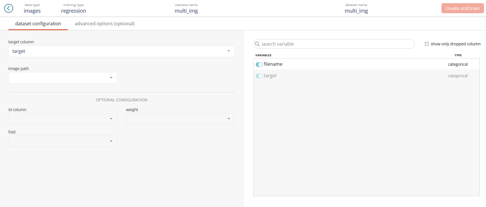
On the left part of the screen, you will be able to fill the same columns than in tabular usecase but you’ll need to add the « image path » feature which link the tabular Data Set and the images folder.
Once done, you can launch the training by clicking on the « create and train » button, located on the top right of the screen:
Optionnally, there are advanced options reachable by clicking the tab in the top bar:

Advanced options
Advanced options do work exactly like for tabular usecases.
Object detection
Like any other images usecase, you need to specify 2 Data Sets (one tabular and one images).
There is a « quick » button that will allow to train a model faster (typically by a factor 5-10) with a little bit less of performance.
Note: While object detection use case can run on CPU’s, the training time will be very long. That’s why we recommand you to have a instance that has GPU in it.
Once this step done you can proceed on cliquing the « configure dataset » button, located on the top right of the screen:
Data Set configuration
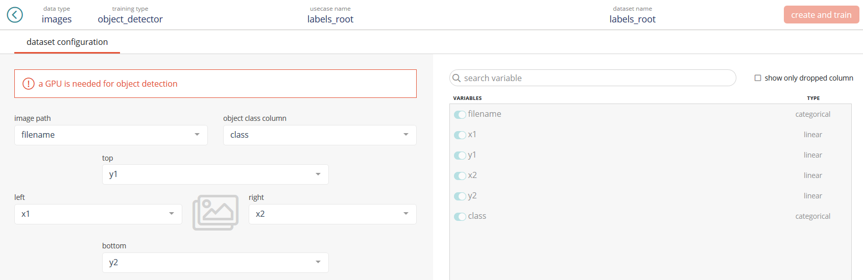
In this usecase type, you’ll need to provide:
- image path: the feature that link the tabular Data Set to the image folder
- object class column: the feature that indicates the category of the object to detect
- top: the top ordinate of the pixel that indicates the bounding boxe in which the object is
- right: the right abscissa of the pixel that indicates the bounding boxe in which the object is
- bottom: the bottom ordinate of the pixel that indicates the bounding boxe in which the object is
- left: the left abscissa of the pixel that indicates the bounding boxe in which the object is
Note: The Data Set shouldn’t contains any other columns than the one required to launche the training
Once done, you can launch the training by clicking on the « create and train » button, located on the top right of the screen: