Data
Navigation
In a project, by clicking on data on the main left navigation, you will enter the data page where all actions and files relative to data are localized. The following 2nd level navigation of the data interface will appear on top of the page.

- Datasets : you can upload .zip or .csv files in this page
- Image folders : you can load .zip files containing images in order to do specific image use cases
- Data sources : by using connectors you can setup data sources in order to generate datasets from database or file server
- Connectors : you can manage connectors to your external databases or file servers in order to apply them on data sources
datasets
Upload a dataset
By clicking on the Datasets button of the dedicated data page menu, you will land on the dataset page.
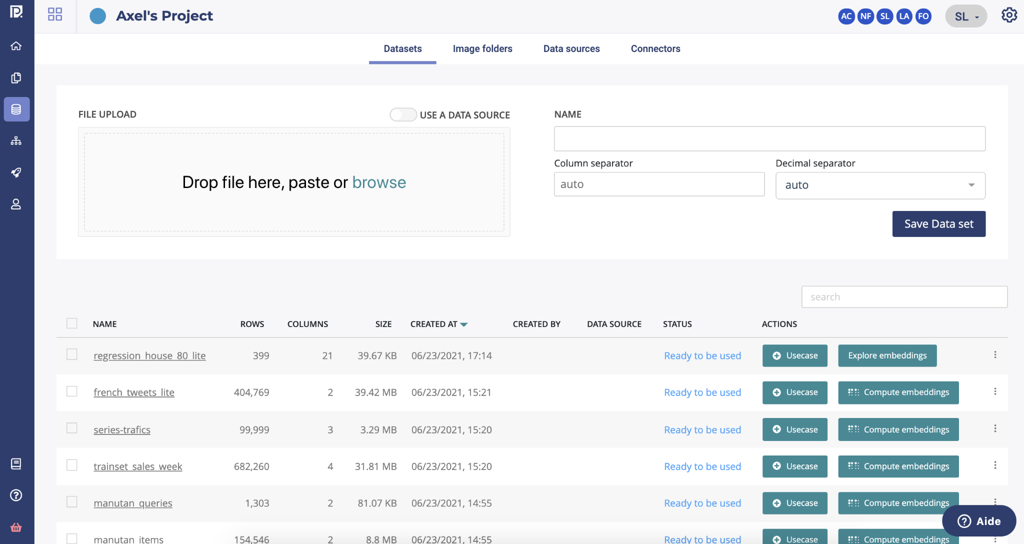
This page allows you to consult all the project datasets uploaded into the application and import new ones by using one of the following methods :
- either from files (CSV or ZIP)
- either from a Data Source at a given time (snapshot)
In order to upload a dataset from a file, you can drag & drop in the dedicated area of your file or click on “Browse” in order to open your computer file explorer. Once your file is selected, you can start the upload by clicking on the “save Data set” button on the right side of the file upload area.
In order to create a dataset from a datasource, you have to use the toggle button “use a data source” and then select a data source from the dropdown list.
When the upload of the dataset is done, the platform will automatically compute information regarding your dataset in order to maximize the automation of machine learning computes. You can follow thanks to the status column on the list the progress of these operations.
dataset statistics pending : pre-computing of dataset information ready to be used : the dataset is ready to be used in the platform dataset statistic failed : the dataset can’t be used in a train, you have to re upload the file drift pre-computing failed : you can train with this dataset but once a model deployed, the drift will be not available
From the dataset table, several actions are possible
Actions
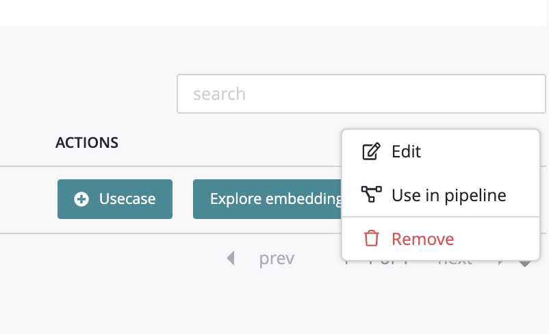
By clicking on the usecase button, you can start the configuration of a training based on the selected dataset. By clicking on the start embedding button, you can launch the dataset analysis computing. Once it is done, the icone in the liste will change for “explore embedding”. By clicking on it you will access to the dataset analysis dedicated page. By clicking on the action button on the right side of the table, you will be able to :
- edit the name of the dataset
- use this dataset into a pipeline
- delete the dataset
Please note that this action button will be also available into a dataset page.
Datasets informations
Navigation
Once your dataset is uploaded and computed into the platform, you will be able to access information about it by clicking on your dataset on the list.
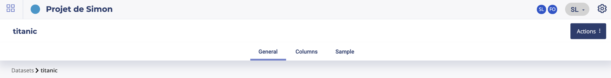
Three menu regarding the dataset are available allowing you to understand better your data
- General : general information about your dataset
- Columns : information about features of your dataset
- Sample : a sample visualisation of your dataset
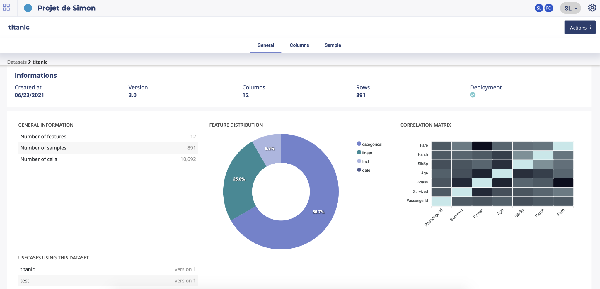
General
On the general screen of a dataset you will find generic information about your dataset such as the number of columns, number of samples and number of cells or the usecases using this dataset. Two graph are also displayed showing : * the feature distribution regarding the feature type (linear, categorial, date or text). This distribution is automatically calculated when uploading a dataset into the platform * correlation matrix showing the correlation coefficients between variables. Each cell in the table shows the correlation between two variables
You will also have on the bottom of the screen the list of usecases trained from this dataset.
Columns
By clicking on the column button on the top menu you will find a listing of all the dataset features, their role (categorial, linear, text or date) and the percentage of missing value for each feature
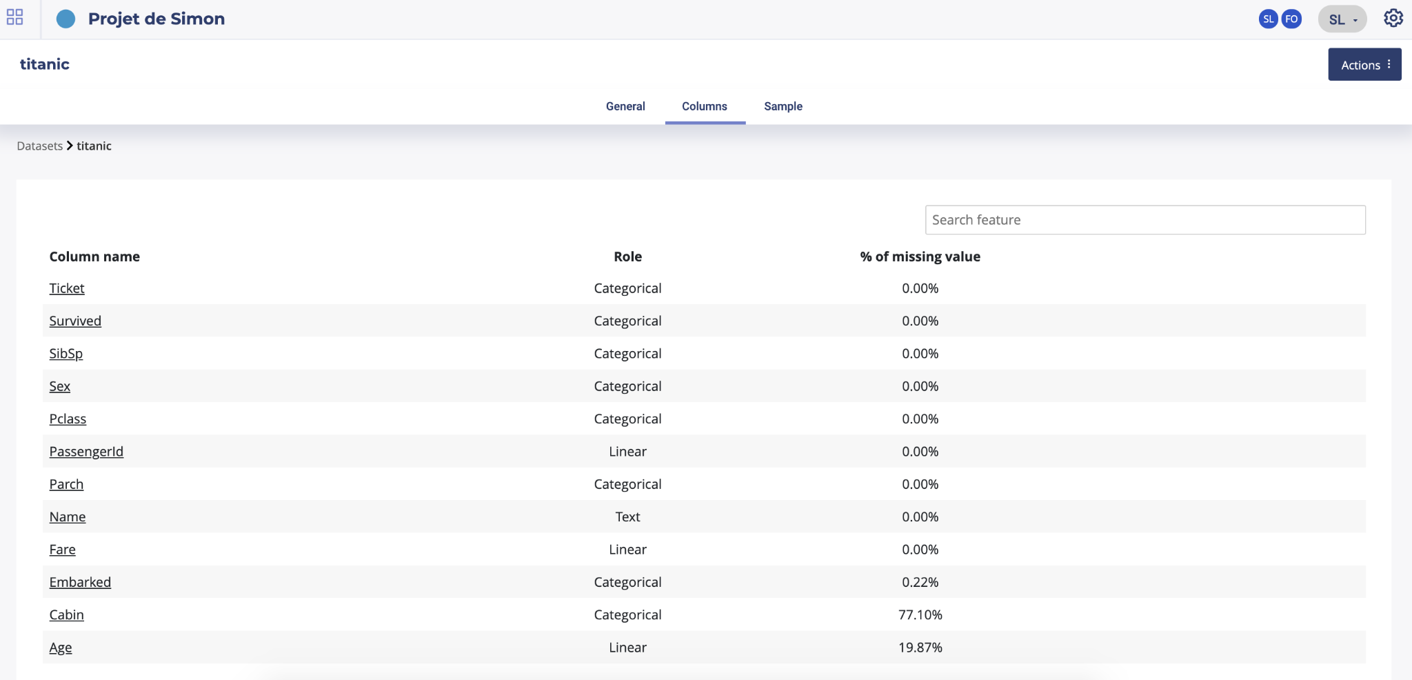
image alt text
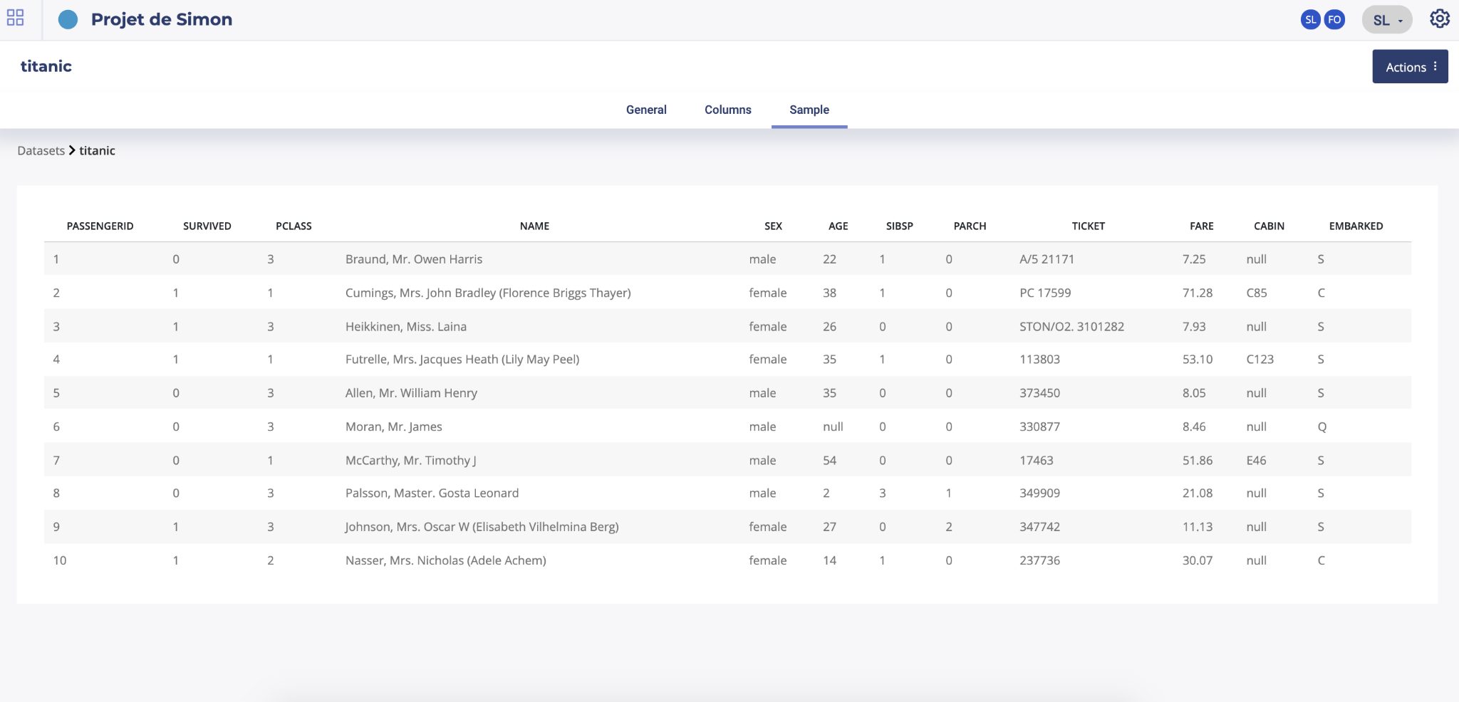
Sample
By clicking on the sample button, a sample of 10 rows of your dataset will be displayed.
Dataset analysis
Introduction
The Data Explorer is a specific module that aims to detect similarities between samples of your dataset. It uses a combination of Dimension reduction algorithms for representing your dataset into a vector space, sometimes called embedding By using it, you’re being able to :
Visually observe cluster see which samples are the most similar to a selected one, for example a Customer in his buying habits See in which population a given feature, like expenses, is present or higher Have a global view of your data
The Data explorer is often used as a pre-analysis of datasets, as it uses an unsupervised algorithm, but it can be used as a standalone feature. Once the embedding has been generated you can request them by API or download them for use in a third party tool like Excel.
Start a dataset analysis
Two possibilities in order to launch the explorer. By clicking on the “start embedding” on the dataset list or, after opening a dataset page, by clicking the actions button on top of the screen and clicking on “start embedding” .
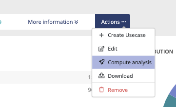
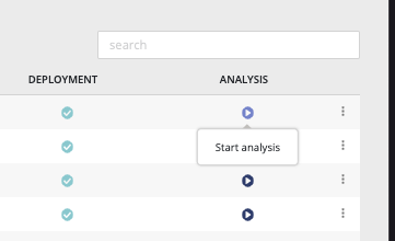
Compute embedding will take more or less time regarding the size of your dataset. Once the computing is done, you will see on the list an eye icone and, on the dataset page on the actions button, the compute analysis button will be replaced by an “explore embedding” button. By clicking on one of these buttons, you will enter into the dataset analysis interface.
The explorer
The Data Explorer is now accessible and will give you a visual representation in 2 or 3 dimensions of the selected Data Set. This representation is a dimension reduction constrained to 2 or 3 dimensions, applied on the embedded vectors, that may be of a higher dimension. There are five important sections in the data explorer.
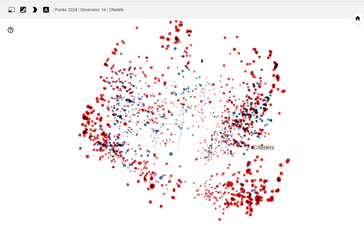
- Graphical projection
The main screen is a visual representation of the dataset. Each point is a sample of your dataset ( up to 5000 ). You can pan and zoom and if you click on a point, or use the selecting box tool, some more info is displayed.
In this representation, points are grouped by similarities as much as possible, meaning that if two points are near in this space, the samples share some important similarities.
The nature of the displayed information are selected on the section (3)
- Search and similarities
The second section is a dynamic list of similar sample.
You can search any sample from any feature. For example if your dataset has an index with name, you can search a sample by using its name but you can too search all the sample that have « RPG » as type or « 5 » for size.
Once a sample is selected, it and a list of similar are is highlighted in the main section. They can be further isolated by clicking on the « isolate N points » button on top of the section.
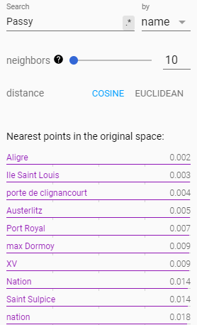
image alt text
The number of similar samples to display can be choosen with the « neighbors » slider
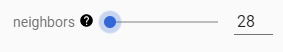
image alt text
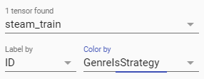
- Labels
Section 3 main purpose is to set labels displayed in section 1. Here you can set :
the label displayed above each point
the feature use for coloring each point :
- Segmentation and clustering
Section 4 is all about Segmentation and clustering your samples.
Here you can choose an algorithm and tune its parameter to display the most similar point together. Thus, you can start to observe sample clusters, or segments of data that represent big groups that share important similarities.
Yet, as we try to project a lot of dimensions in a smaller space (3D or 2D), note that this algorithm is just for displaying and shaping human decision. A lot of the process is a little bit subjective and further conclusion should be driven by a supervised algorithm.
Anyway, here you can choose between 3 algorithms :
- PCA : the quickest and simplest algorithm. Clicking on the PCA tab immediately led to a 3D representation of your samples. Yet, this is a very simple algorithm that only shows sample variability along 3 axes. You can find more information about PCA on Wikipedia
- t-SNE : once you click on the t-SNE tab, a process of convergence is launched. t-SNE is a very time consuming algorithm but that can lead to very accurate segmentation. You can change its parameters and click on the « Stop » button then « Re-run » it. But in most cases it’s better to already know this algorithm to use it. You ca find more information about t-SNE on Wikipedia
- UMAP : UMAP is a good alternative to t-SNE and PCA. Quicker than t-SNE , it offers better results than PCA. THe only parameters is « Neighbors », that change the size of clusters. The more neighbors you ask for, the bigger the cluster. You can find more information about UMAP on Wikipedia.
We recommend using UMAP in most cases.
- API informations
The 5th part is only about API information.
When launching a dataset Analysis, the platform builds an embedding of the dataset, namely, it projects each sample of the dataset to a vector. This embedding is attached to the dataset and can be retrieved with the dataset ID. Then you can use it for running any mathematical operation, in most cases a distance, that can be run on vectors.
Section 5 of the tools gives you the Id of your dataset :
image alt text
With it you can access several URL :
- GET https://.prevision.io/api/datasets/files//download : get the original dataset
- GET https://.prevision.io/api/datasets/files/ : JSON info about your dataset
- GET https://.prevision.io/api/datasets/files//explorer : JSON info about the embeddding
- GET https://.prevision.io/api/datasets/files//explorer/tensors.bytes : numpy files of embeddings
- GET https://.prevision.io/api/datasets/files//explorer/labels.bytes : tsv files of labels
The embedding files (tensor.bytes) is a numpy float 32 file whom shape is in the json file if explorer URL. You can read it with the following python code for example
req = Request('https://<YOUR_DOMAIN>.prevision.io/ext/v1/datasets/files/<DATASET_ID>/explorer/tensors.bytes')
req.add_header('Authorization',<YOUR_TOKEN> ) #get YOUR_TOKEN in the admin page
content = urlopen(req).read()
vec = np.frombuffer(BytesIO(content).read(), dtype="float32").reshape(u,v) # u,v is the shape gotten in /ext/v1/datasets/files/<DATASET_ID>/explorer
print(vec.shape)
Please note that you can use SDK’s functions in order to simplify this process.
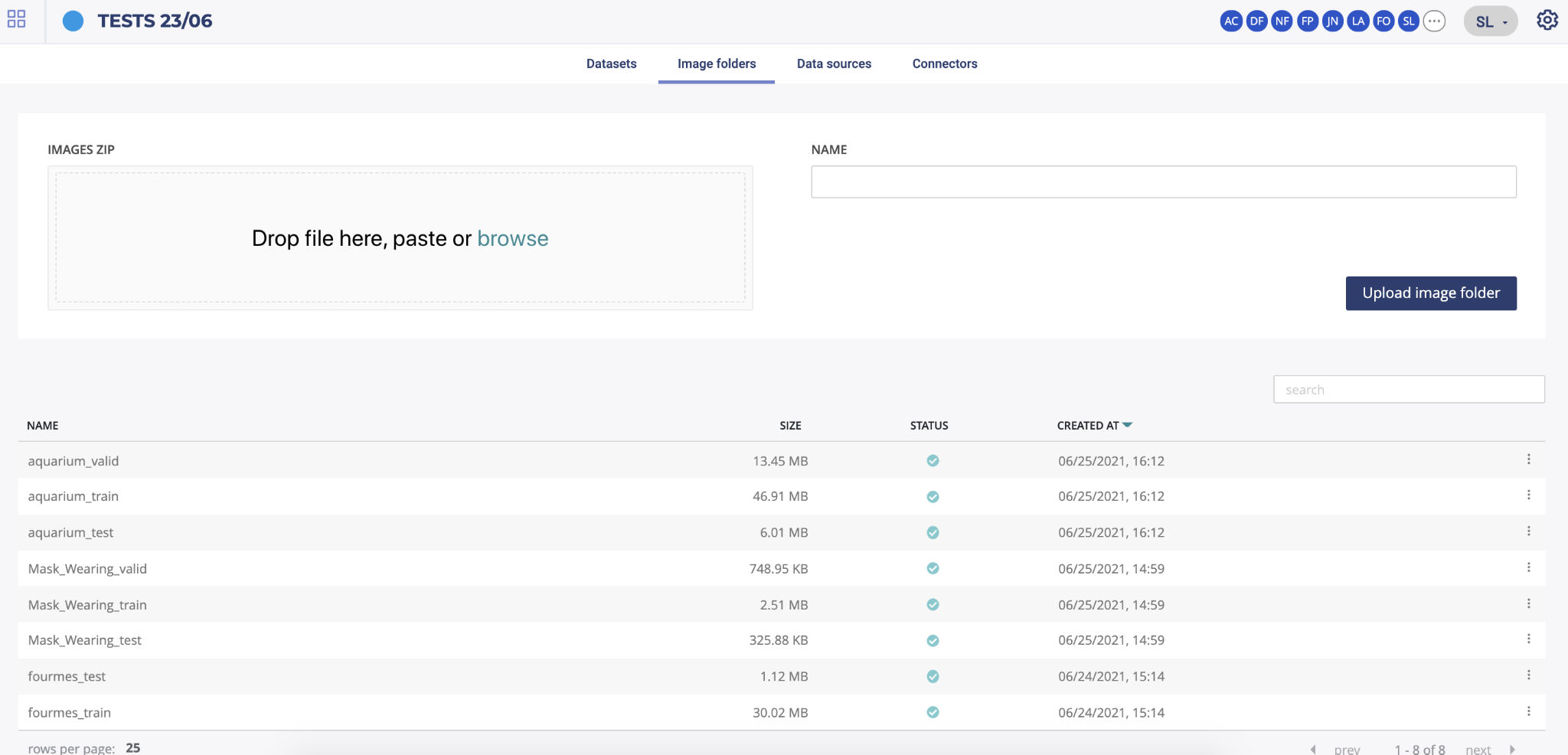
image folders
In order to train image use cases you will have to upload images using a zip file. By drag & drop a zip file in the dedicated area you will be able to load your image folder. All images folders uploaded into your project will appear in the list under the drag & drop section.
It is recommended to use an images dataset whose total volume does not exceed 4 GB. We invite you to contact us if you want to use larger datasets.
By clicking the action button on the list you will be able to :
- edit the name of your image folder
- delete your image folder
Connectors
In the Prevision.IO platform you can set connectors in order to connect the application directly to your data spaces and generate datasets. Several connector types are available :
- SQL databases
- HIVE databases
- FTP server
- Amazon S3 datastore
- GCP
By clicking on the “new connector” button, you will be able to create and configure a new connector. You will need to provide information depending on connector’s type in order for the platform to be able to connect to your database/file server.
Note
TIPS : you can test your connector when configured by clicking the “test connector” button.
Once connectors are added, you will find under the new connector configuration area the list of all your connectors. You can, by clicking on the action button :
- test the connector
- edit the connector
- delete the connector
Once at least one connector is well configured, you will be able to use the data sources menu in order to create CSV from your database or file server.
Data sources
In order to create datasets, you first need to configure a data source using connector information. To do this, click on the data sources menu and select the configured connector in the dropdown list. Depending on the connector type, you will have to configure the data source differently.
When your data source is ready, in order to generate a dataset from it, you have to go to the datasets page, enable the toogle button “use a data source” and select your data source from the dropdown list.
SQL data sources
Once a SQL connector is selected, you will have to choose first the database you want to use. Then, two different methods are available in order to configure your data source :
- by selecting a table
- by clicking the “select by query” button and entering a valid SQL query